Lab 3: Rediscovering Trails in National Parks (4.5 pts)#
Read before proceeding#
The questions for this lab are embedded within the instructions.
Each question carries specific points, clearly indicated alongside it.
The questions might have subsections within them.
The total score for this assignment is 10 points. Your final grade will be scaled from the total points you earn out of the maximum possible score to fit within a 0 to 10 scale.
When working on a lab, always create a dedicated folder for it and store all related files within that specific folder. For instance, avoid saving intermediate files in the
C:/Documentsdirectory; keep all materials organized and together.Create a word document and name it as
Lab-3-answers-YOURLASTNAME.docx. Insert each questions provided in this document and write down your answers for each questions. Upload the.docxfile in Canvas. Do NOT upload a.pdfof the document.Upload any additional file(s) required by this instructions in Canvas. You will find specific list of deliverables at the end of this page.
You do not have to upload any large ArcGIS Pro Project (
.asprx) file unless explicitly mentioned in the instructions.
Due Date#
Oct 3, 2024 10:00 PM CDT
Background#
The natural landscapes of national parks offer a unique blend of topographical diversity and ecological richness. Trails winding through these parks often lead to high vantage points that provide breathtaking views and immersive experiences in nature. Understanding these landscapes requires an integration of various geospatial analyses to assess both the physical terrain and the ecological attributes.
In this lab, you will analyze hiking trails to identify those with the highest average slope and the highest peaks. Slope is a critical factor in assessing trail difficulty, as trails with greater slopes require more physical effort and can be more challenging for hikers. Trails that reach high elevations provide scenic views but may also be more strenuous. By analyzing slope and elevation data along the trails, you will determine which trails are the steepest and which lead to the highest points, helping to evaluate their difficulty and appeal for different types of users.
We will be working with Rocky Mountain National Park in Colorado. One of my personal favorites.
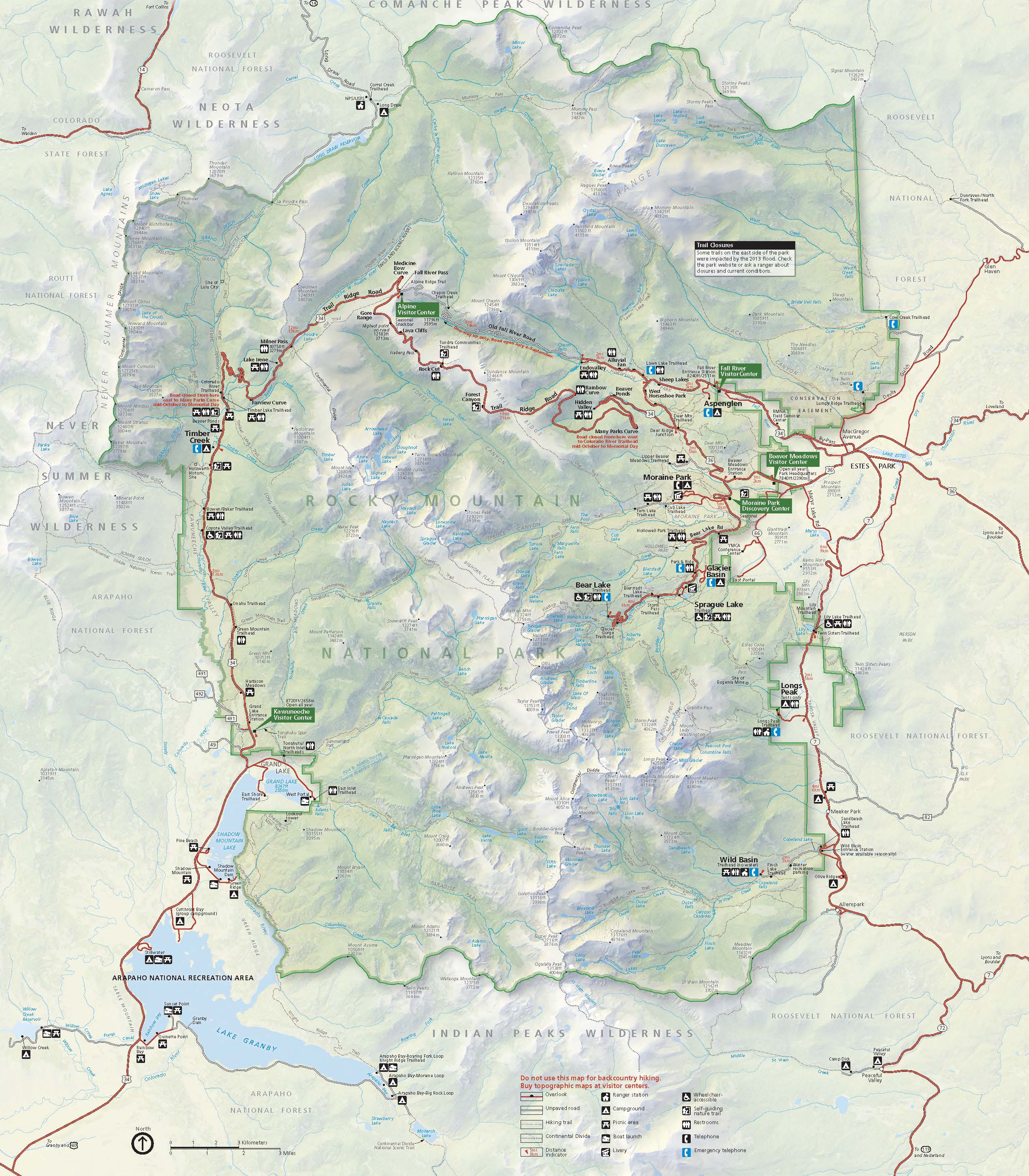
Fig. 71 Rocky Mountain National Park Official Map#
Setup ArcGIS Project#
Create an ArcGIS Porject file in your lab directory named as Rocky_Mountain.
Download the data#
You will have to download your own data. Followings are the steps to download your data. We will download Rocky Mountain National Park boundary, trail, and corresponding DEM data.
Go to https://public-nps.opendata.arcgis.com/, click the search button on the top right corner and type “rocky mountain national park boundary”.
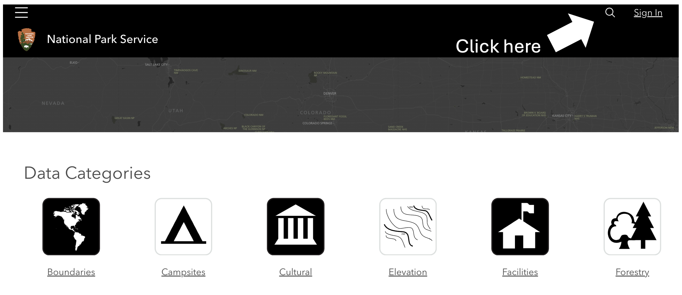
Fig. 72 NPS website#
Click the
Rocky Mountain National Park - Boundary Polygonand download it as a Shapefile in your Lab 3datadirectory.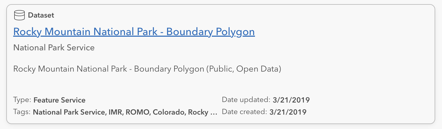
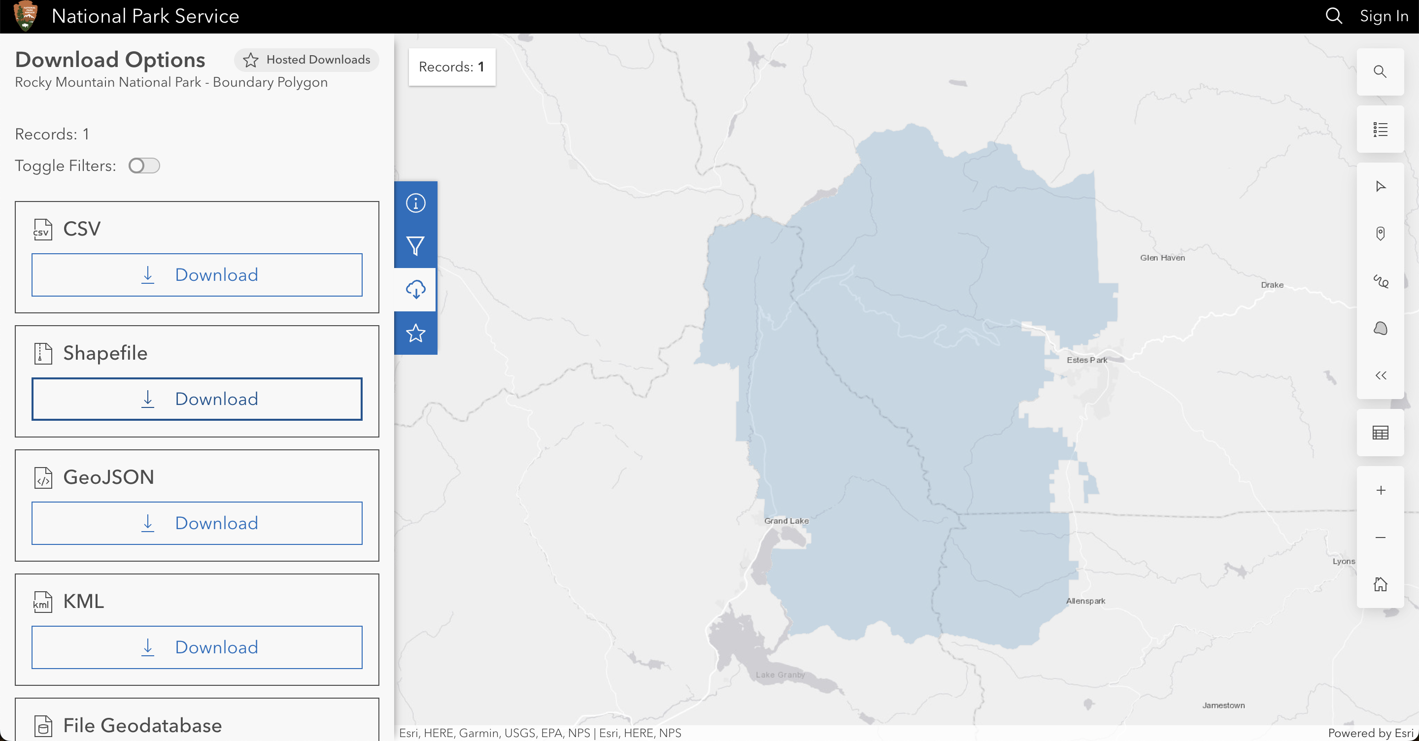
Fig. 73 RMNP Boundary shapefile download#
Go to https://public-nps.opendata.arcgis.com/ one more time, click the search button on the top right corner and type “rocky mountain national park trails”. You should see a
Rocky Mountain National Park - Trailslabel and download it as a shapefile.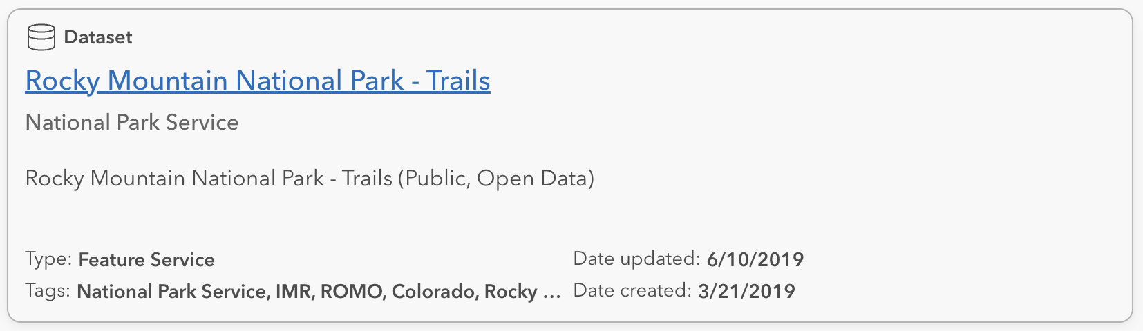
Fig. 74 RMNP Trails shapefile download#
Go to https://apps.nationalmap.gov/downloader/, which is the official site to download USGS open source data. Here you can find a lot of good curated dataset published and/or maintained by USGS. We want to download the Digital Elevation Model (DEM) products from here.
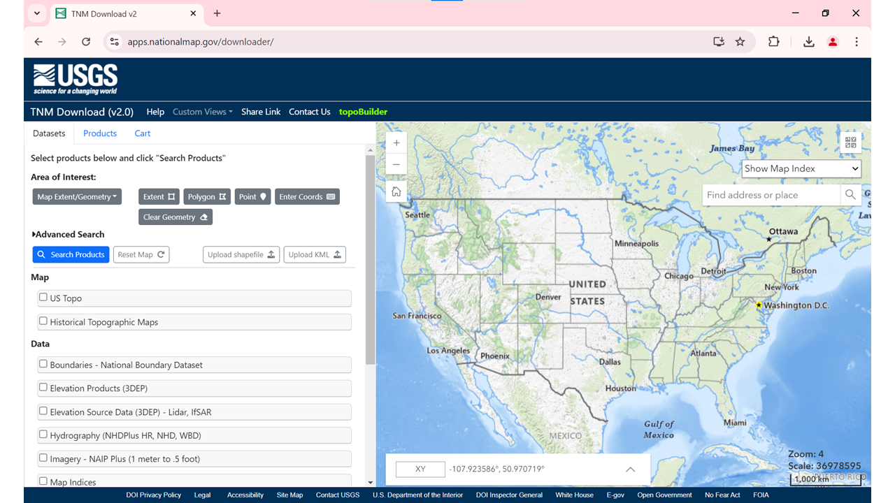
Fig. 75 The National Map Downloader#
There are multiple ways to download data, i.e., Extent (whatever extent the map is in the right side section), Polygon (you can upload your own polygon), Point, Enter Coords (the extent of your area of interest). We will use the
Enter Coordsoption to insert the RMNP boundary extent information.
Fig. 76 Extent window#
Now go to you ArcGIS Pro project and click the properties of the
Boundary_(Polygon)(which is the RMNP boundary) layer. To find the Extent of this layer, clickSourceon the left side pane, and then clickExtent. You will see that the Extent information (Top, Bottom, Left, Right) are available in meters as the layer is in a projected coordinate system. On the other hand, the National Map requires the extent to be in geographic coordinate system or latutide/longitude values rather than meters. Therefore, we need to change the projection of this layer to a geographic coordinate system. Find the Project tool in the Geoprocessing tools and create a feature class named asBoundary_Polygon_GCSin the project geodatabase withGCS_WGS_1984system. Click the little globe icon in theOutput Coordinate Systemparameter and selectWGS 1984from theGeographic Coordinate Systemoptions.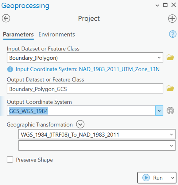
Fig. 77 Projecting boundary polygon#
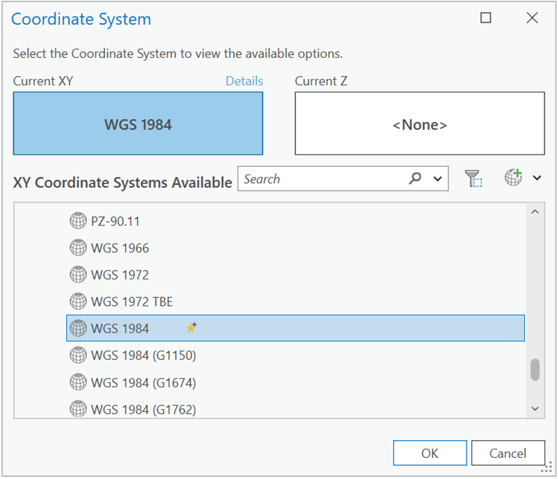
Fig. 78 Finding WGS coordinate system#
Now open the properties of
Boundary_Polygon_GCSlayer and locate theExtent. Make sure it matches with the following information.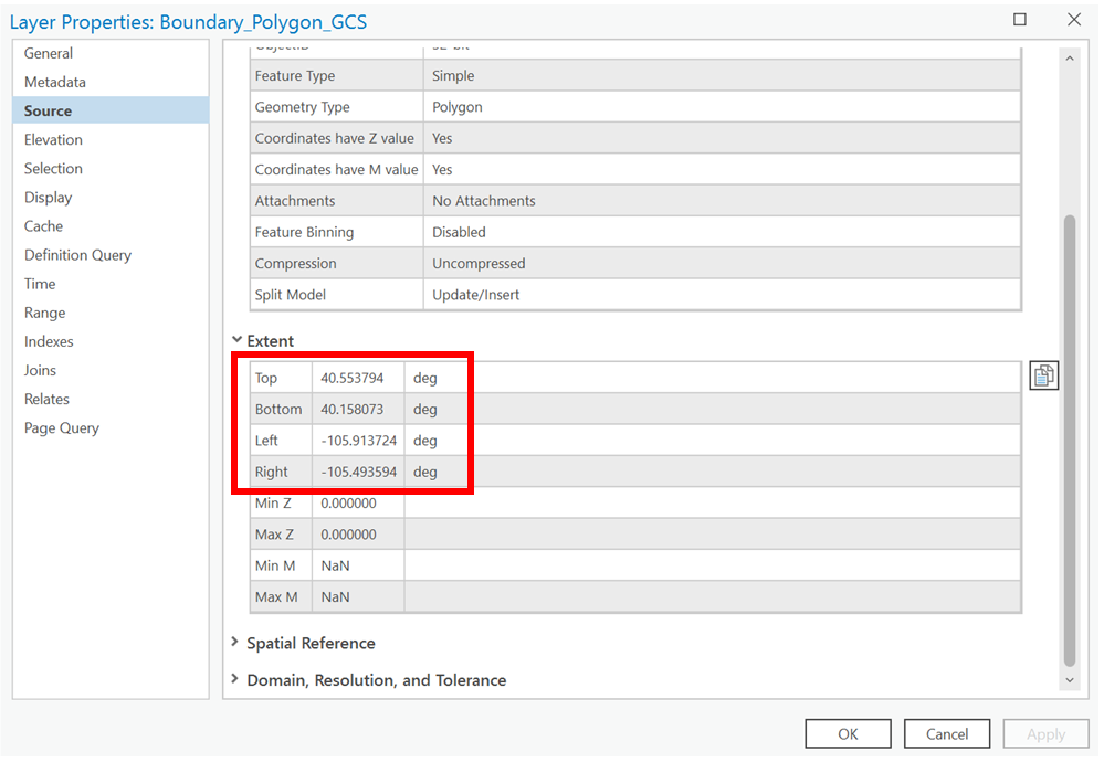
Fig. 79 RMNP Extent#
Top: 40.553794 Bottom: 40.158073 Left: -105.913724 Right: -105.493594
In your browser, clear the Extent window if it was open. First, select the dataset we need to download. We will be downloading a 10-m resolution DEM from USGS, which is a very common and good DEM data within US. However, the 10-m resolution is an approximation from 1/3 arc second resolution. Check the
Elevation Products (3DEP)in the left side pane on theDatasection, then select the1/3 arc-second DEM(Current).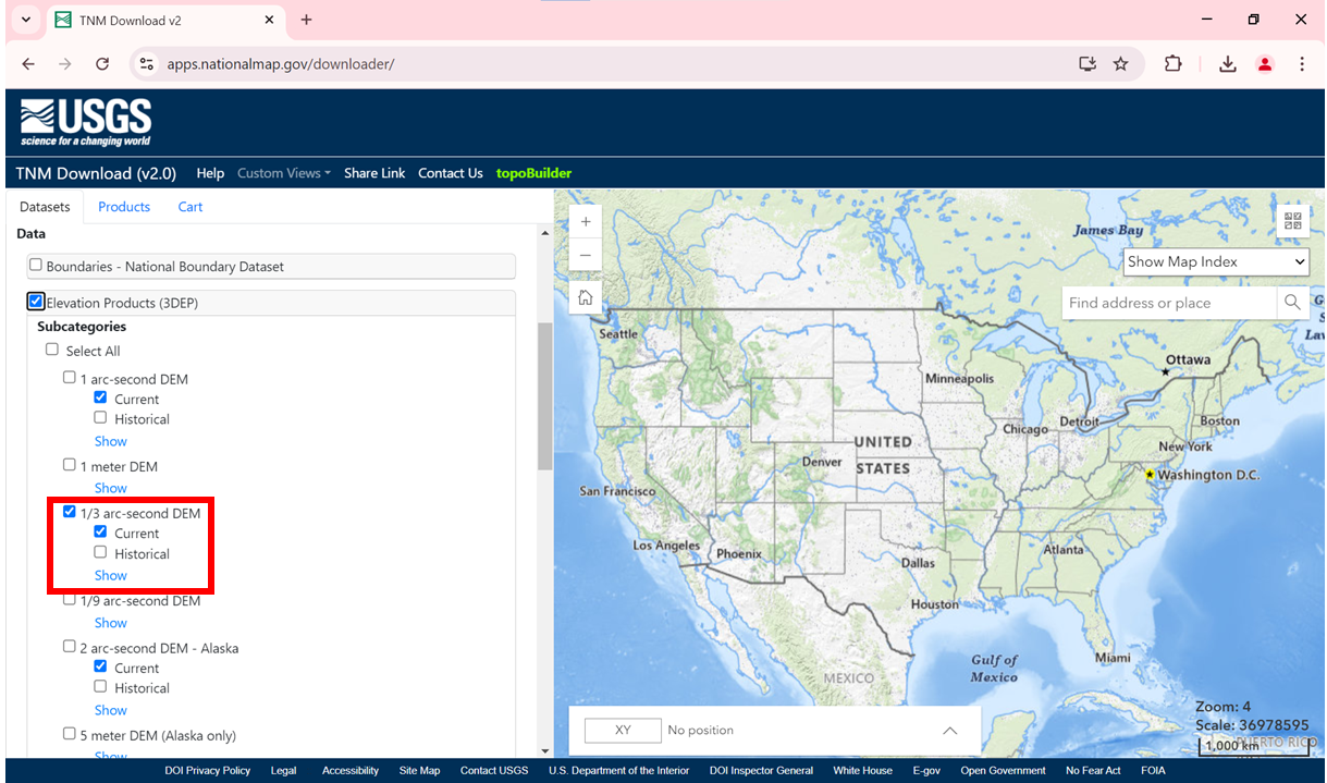
Fig. 80 Selecting data#
Now, we need to provide the Extent information. Make sure the Extent information of your RMNP Boundary in geographic coordinate system is handy in ArcGIS Pro. Then clicl the
Enter Coordsbutton on theArea of Interestsection of the window on the left. Now provide the extent information correctly with absolute precision. The Xmax, Xmin, Ymax, Ymin are actually Right, Left, Top, and Bottom, respectively in terms of ArcGIS Pro’s Extent information. It should look like below and once you are satisfied, clickAdd to Map.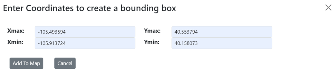
Fig. 81 Providing extent information#
After adding the extent, there will be a AOI drawn on the right side map. If it makes sense, click
Search Products.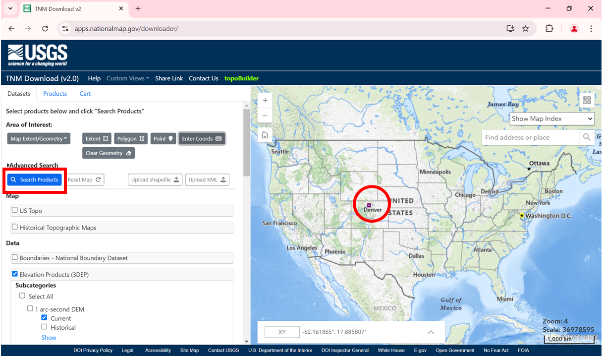
Fig. 82 Showing extent on the map#
There should be one product as the result. Make sure it matches with the following. Click ``Download Link (TIF)
to download it as a tif file. You can also clikFootprintto see the footprint of the DEM on the right map, clickZoom Toto interact with the DEM on top of the topographic basemap. Download the DEM in yourdata` directory.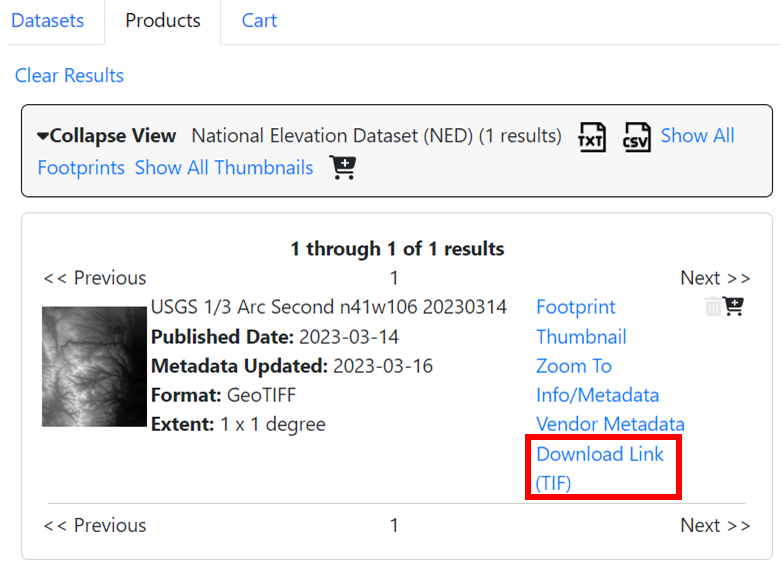
Fig. 83 Search results of DEM#
Workflow using ArcGIS Pro#
Explore the datasets#
Insert the RMNP Boundary shapefile that you downloaded.
Question 1
a. What is the total area of the RMNP in Square Kilometers? <1 pt>
Insert the RMNP Trails shapefile you downloaded.
Question 2
a. What is the total length of trails in Miles within RMNP? <1 pt>
b. How many unique trails are within RMNP? (Hint: if you examine theTRLNAMEcolumn, you will find that there are some Polylines with sameTRLNAME. Therefore, you need to doDissolveof theTRLNAMEso any trail with same name will be merged together. While doing so, also calculate theSumstatistic of theLength_Milefield, so you get the total length of each unique trail in Miles.) <3 pt>
c. Which trail is the longest and what is its length? (Hint: Remember to use the dissolved trail feature) <2 pt>
d. What is the mean and median length of trails in RMNP? (Hint: Remember to use the dissolved trail feature) <2 pt>
e. Is the distribution of trail length normal or skewed? If skewed, positive or negative? (Hint: Remember to use the dissolved trail feature) <2 pt>Insert the
USGS_13_n41w106_20230314.tifyou downloaded. Explore the DEM. Look at its values in the table of contents which is in Meters. Let’s convert this to Feet. The conversion formula for meter to feet is to multiply the raster data by a constant value of3.28084.Question 3
a. Create a DEM where the unit of the elevation is in Feet. Save it in the default geodatabase without mentioning any file extension. This will create a native ESRI Grid format raster data. (Hint: Use Raster Calculator from Spatial Analyst extension) <3 pt>
b. What is the maximum and minimum value of the elevation for this entire raster in Feet?<3 pt>
Clip the DEM to analysis boundary#
Since the DEM is quite larger than the RMNP boundary, we do not need the entire DEM for our analysis. Therefore, it is better to clip or mask the DEM by the RMNP boundary extent. To do this, find the Clip Raster tool and use the Boundary_(Polygon) as the Output Extent to clip the DEM_Feet raster. Make sure the output data is saved in the default geodatabase as DEM_Feet_Clip. Also check the Maintain Clipping Extent at the end.
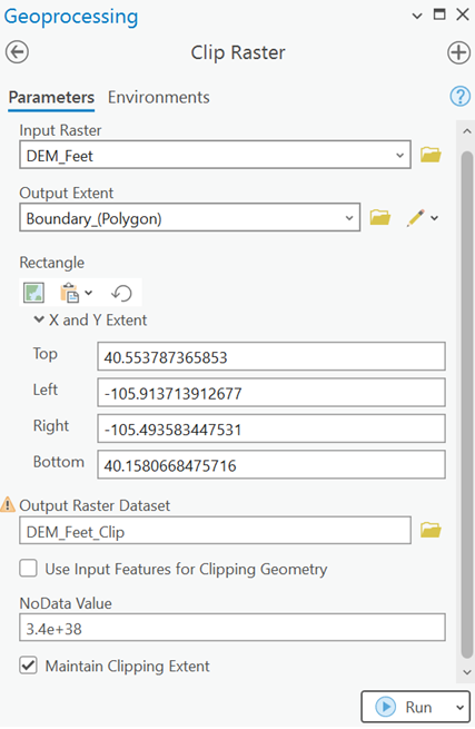
Fig. 84 Clip raster#
Find the peak points within trail lines#
To find the highest/peak points within the trails, we can use many different approaches. Here is a simple approach:
First, we can generate equal distant points on top of the line(s)
Then, we use those points to extract the elevation values from the DEM
Once we know the elevation of each points, we can find the maximum value for each trails
Then we filter out the top 5 peak points to calculate viewshed.
Find the Generate Points Along Lines (Data Management Tools). Use
Trail_Dissolveas theInput Features, name theOutput Feature ClassasTrail_Pointswithin the default geodatabase, use10 Metersas theDistanceas we know that the USGS DEM is 10 m resolution. Approximating 10 meters interval points will be good enough for our analysis. If you want more precision, you can use smaller number but for this lab, let’s stick to 10 meters. Makse sure to check theInclude end pointsso the starting and ending points are also included in the results.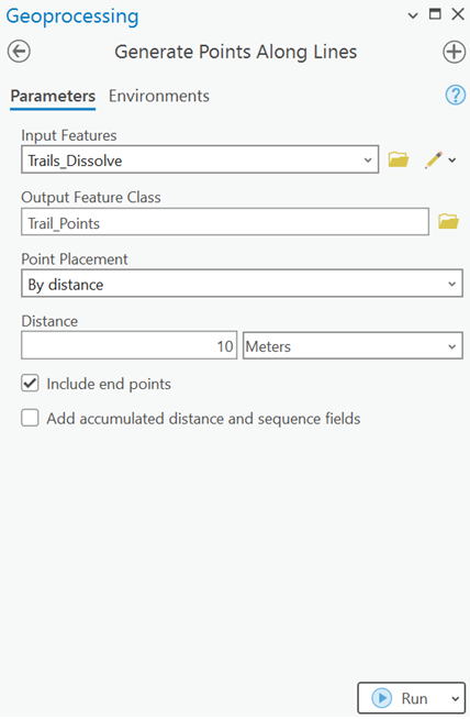
Fig. 85 Generate points along lines#
Question 4
a. How many points you got? (Hint: it should be 54,070 points, if not, something was wrong in your previous steps) <1 pt>
Find the Extract Values to Points (Spatial Analyst Tools). Use the
Trail_Pointsas theInput point features;DEM_Feet_Clipas theInput raster; name theOutput point featuresasTrail_Points_Elevationin the deafault geodatabase.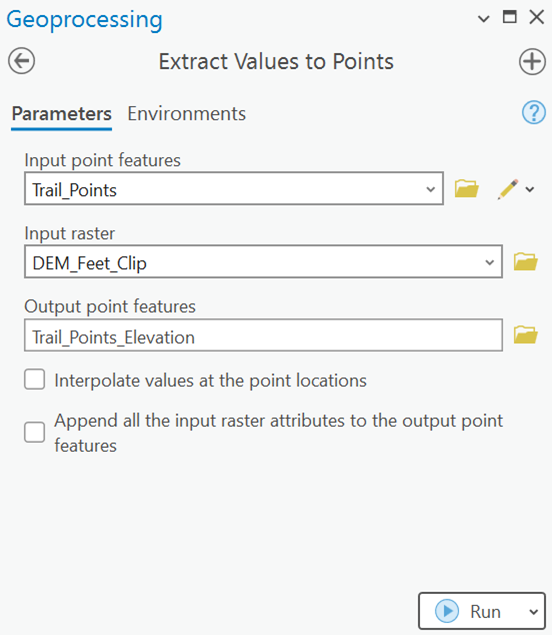
Fig. 86 Extract values to points#
Explore the
Trail_Points_Elevationfeature’s attributes. See that there is an attribute calledRATERVALUwhich includes the elevation in feet underneath each point. Now we need to find out the highest point within each trail.We can use the Dissolve (Data Management Tools to aggragte unique
TRLNAMEwithin each points. Use the following parameters in the Dissolve tool. Make sure you are calculating theMaximumRASTERVALUas theStatistics Fieldsand theDissolve Fieldsis theTRLNAME.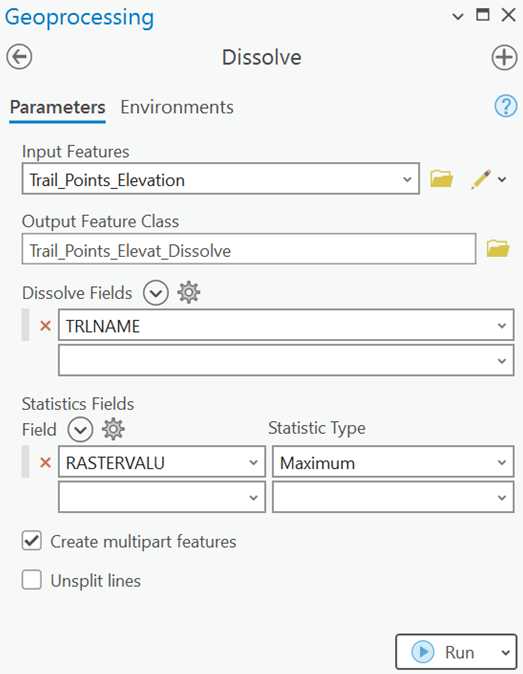
Fig. 87 Dissolve points#
Explore the attribute table of the
Trail_Points_Elevat_Dissolvefeature. See that we have160unique trails only, which makes sense. Now we need to find out the 10 meter interval points of each trail that matches with theMAX_RASTERVALUvalues. To do this, we can join the dissolved points’MAX_RASTERVALUattribute to theTrail_Points_Elevationattrbute by using theTRLNAMEas the join field.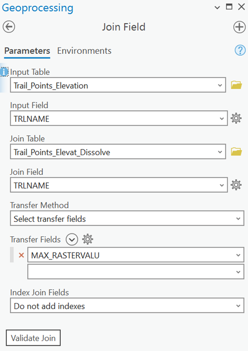
Fig. 88 Join maximum elevation value#
Explore the attribute of the
Trail_Points_Elevationfeature. See that we haveRASTERVALUwhich is the actual elevation value for each point, and theMAX_RASTERVALU, which is the maximum elevation within each trail. The points where the difference between these two attributes are0, are the peak points for each trail. Therefore, create a new field calledELEV_DIFF(Elevation difference) and compute the difference betweenMAX_RASTERVALUandELEV_DIFF. The points that has a value of0would mean that point is the corresponding peak within that particular trail. Now, select the points that has0values in theELEV_DIFFattribute (by using theSelect By Attributes) and export that data to a new feature calledTrail_Peak_Pointsin the default geodatabase (Hint: right click the selected layer, click Data, then Export Features).Question 5
a. How many points you got? <1 pt>
b. If you have done the analysis correctly, then the number of peak points you got should be slightly larger than 160, which is the unique number of trails within RMNP. Why you have got more peak points? <2 pt>Since there are some duplicated trail points in the
Trail_Peak_Pointsfeature, we can use the Delete Identical (Data Management Tools) to remove identical entries from theTRLNAMEattribute.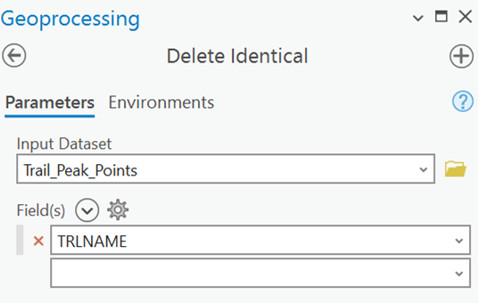
Fig. 89 Delete identical#
Select the top 5 highest peaks from the
Trail_Peak_Pointsfeature and export it seperately asTop_Five_Peak_Trails.
Calculate slope of the DEM#
Use the Slope (Spatial Analyst) tool to calculate slope of the DEM. Save it as Slope in the default geodatabase.
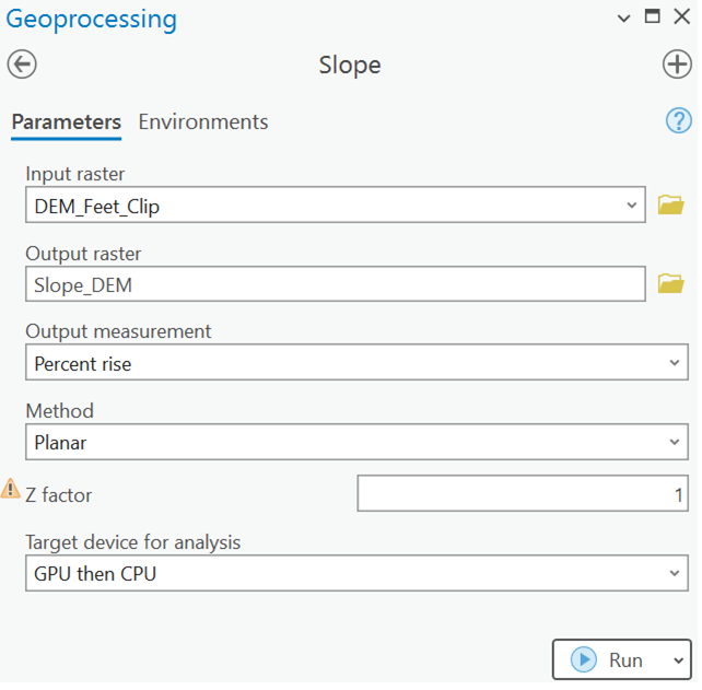
Fig. 90 Slope#
Find which trails have the highest mean slope#
Find Zonal Statistics as Table (Spatial Analyst) to calculate the mean slope value for each trail (Trails_Dissolve).
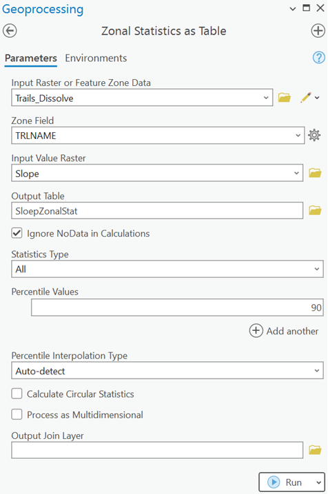
Fig. 91 Zonal Statistics as table#
Question 6
a. Zonal statistics as table will give you a table within ArcGIS. Join this zonal table with the Trails_Dissolve layer and identify the top five trails that has the highest mean slope. <2 pt>
Question 7
Create a map with the following items:
a. An appropriate basemap of the Rocky Mountain National Park with boundary
b. 5 Trail lines that has the highest peaks
c. On top of the 4 highest peak trails, show the corresponding peak points with its elevation as label
d. Top 5 trails that shows higher average slope
e. The trails that has highest peak and highest slope should not have same color
f. Any other necessary items
<10 pt>
Deliverables#
Your completed
Lab-3-answers-YOURLASTNAME.docxThe final map you generated
Answers#
Question 1
a. 1080
Question 2
a. 334.97
b. 160
c. Beaver Meadows / Moraine Park Complex Trail, 15.07 Miles
d. Mean: 2.08 Miles and Median: 1.51 Miles
e. Not normal, positively skewed.
Question 3
a. No Answer
b. Maximum is 14252.1 feet and minimum is 4837.17 feet.
Question 4
a. 54,070
Question 5
a. 177
b. Because of the 10 meters interval during the generate points step. Since we included the end points when generating points along lines, there could be very adjacent points that share the same elevation cell from the DEM. So sometimes more than one points were sharing the maximum elevation cell resulting in more peak points.