Lab 4: Watershed and Drainage Modeling from DEM (4.5 pts)

Lab 4: Watershed and Drainage Modeling from DEM (4.5 pts)#

Read before proceeding#

The questions for this lab are embedded within the instructions.
Each question carries specific points, clearly indicated alongside it.
The questions might have subsections within them.
The total score for this assignment is 10 points. Your final grade will be scaled from the total points you earn out of the maximum possible score to fit within a 0 to 10 scale.
When working on a lab, always create a dedicated folder for it and store all related files within that specific folder. For instance, avoid saving intermediate files in the C:/Documents directory; keep all materials organized and together.
Create a word document and name it as Lab-3-answers-YOURLASTNAME.docx. Insert each questions provided in this document and write down your answers for each questions. Upload the .docx file in Canvas. Do NOT upload a .pdf of the document.
Upload any additional file(s) required by this instructions in Canvas. You will find specific list of deliverables at the end of this page.
You do not have to upload any large ArcGIS Pro Project (.asprx) file unless explicitly mentioned in the instructions.

Background#

Watershed and drainage from DEM#

Watershed and drainage delineation from a Digital Elevation Model (DEM) involves identifying the boundaries of areas where all precipitation flows to a common outlet, such as a river or lake. A DEM represents the elevation of terrain and serves as the basis for determining how water moves across the landscape. By analyzing the flow direction and accumulation within the DEM, it becomes possible to outline watersheds and extract stream networks. This process allows us to understand the natural pathways that water takes over the terrain, highlighting critical areas for resource management.

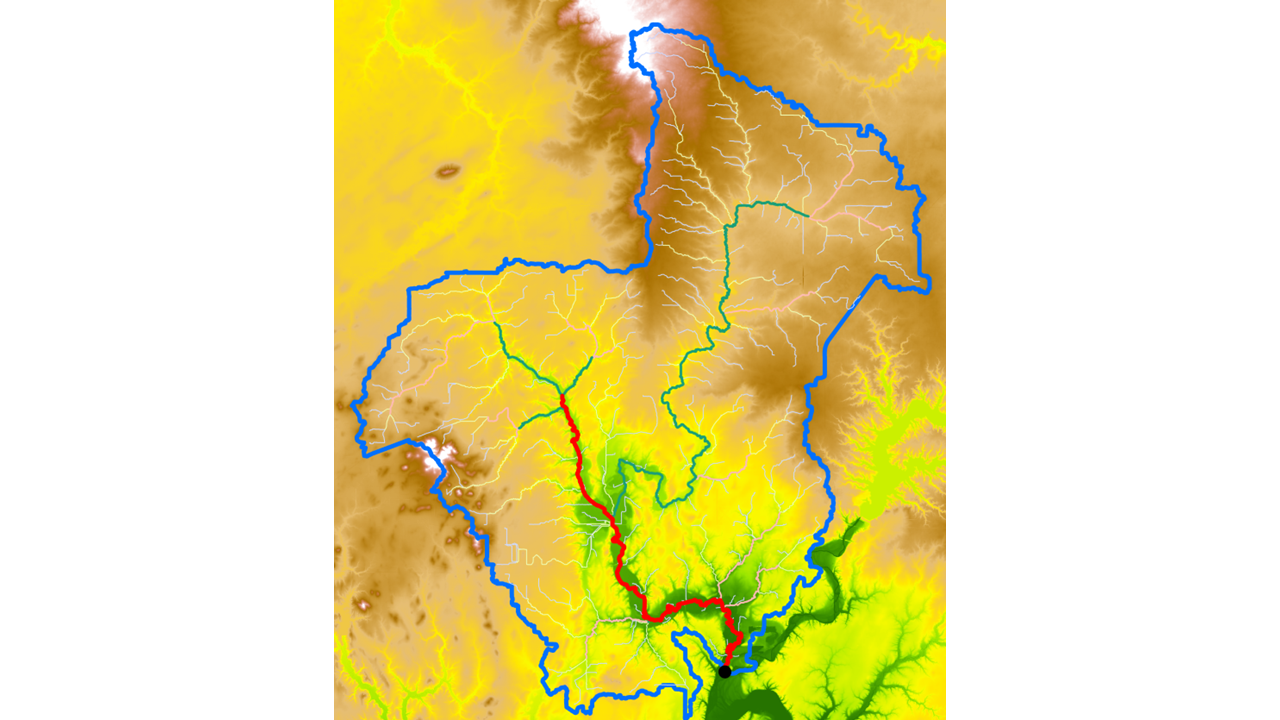
../../_images/fig-4-1.png — Fig. 92 Watershed delineation#

Learning expectations#

Learning watershed and drainage delineation from DEM is important for geospatial analytics because it provides key insights into the movement of water across landscapes, which is crucial for environmental planning, agricultural management, and urban development. It enables us to model hydrological processes, identify potential flood zones, and support decision-making in land and water conservation. By learning these methods, you will also be able to perform raster analysis on top of DEMs, applying techniques like flow direction and accumulation to solve real-life problems such as predicting flooding, planning irrigation systems, and managing natural resources more effectively. Understanding these concepts is essential for professionals who want to analyze how natural systems interact with human activities and use spatial data to make informed, sustainable planning decisions.

Overall goals#

You will be given a 10-m resolution DEM for an area in Illinois (Robinson Creek in Shelby County) and a corresponding Pour Point or Outlet Point in the lower elevation area of the DEM. Your general tasks are:

Create stream or drainage lines from the DEM
Generate a watershed boundary or catchment area or basin given the Pour Point or Outlet

General workflow for watershed and drainage delineation#

We have learned from the lecture that the general workflow for delineating drainage and watershed involves several tools. The logical workflows include:

Hydrological conditioning of the DEM: This is also known as Fill, Pit Filling, Sink Filling, Depression Removal, and so on. The objective is to fill up any holes or depressions or sinks in a DEM so water can smoothly flow downstream.
Flow Direction: Calculate the direction of water flow for each cell by utilizing the depressionless DEM.
Flow Accumulation: Calculate the amount of water flow into each cell by utulizing the Flow Direction raster.
Streamline or drainage delineation: This process involves several small tasks. First, we need to find out a stream raster using a condition of threshold, then calculate the stream order (learn more about stream order) raster, and finally convert the stream order raster to a streamline vector.
Watershed boundary: Watershed boundary delineation require a flow direction raster and the location of pour point, which gives us the area from which all the water flows into that outlet.

Data#

The data for this lab can be downloaded from https://sluedu-my.sharepoint.com/:u:/g/personal/sourav_bhadra_slu_edu/EeweXogS3m9GlOSqsgTzDuUBKOkhq_qK-LHVGkzMoNHgmw?e=rywEnf. If you are logged into your SLU account within your browser, you should be able to download the data. This is a zipped folder and it contains two data, i.e., a RobinsonCreek_DEM.tif as the DEM at 10m resolution, and a PourPoint.shp data as the outlet point location.

Note: The DEM data was downloaded from Illinois GIS Data Clearinghouse. There are often state-maintained GIS data clearinghouses where you can get publicly available GIS data in both vector and raster format. These are usually maintained by the corresponding state universities. For example, University of Missouri Columbia maintains the Missouri Spatial Data Information Service (MSDIS), which is the clearinghouse for the Missouri data. The DEM data I downloaded from the Illinois GIS Data Clearinghouse was derived from the llinois Height Modernization (ILHMP) program. These are LiDAR data at very high-resolution (aroun 3.5 m). However, due to the processing time limitation for our labs, I have reduced the extent of the DEM and resampled the spatial resolution to 10 meters.

Create a lab directory in your local drive and open a new ArcGIS Project within it.

Workflow using ArcGIS Pro#

Hydrologic conditioning of DEM or Filling#

Insert the RobinsonCreek_DEM.tif into your map.
Find Fill (Spatial Analyst) tool and create an output named Fill in the default geodatabase. Since we are saving it in the geodatabase, we can rely on the default ESRI grid as the raster format which does not require an extension within a geodatabase.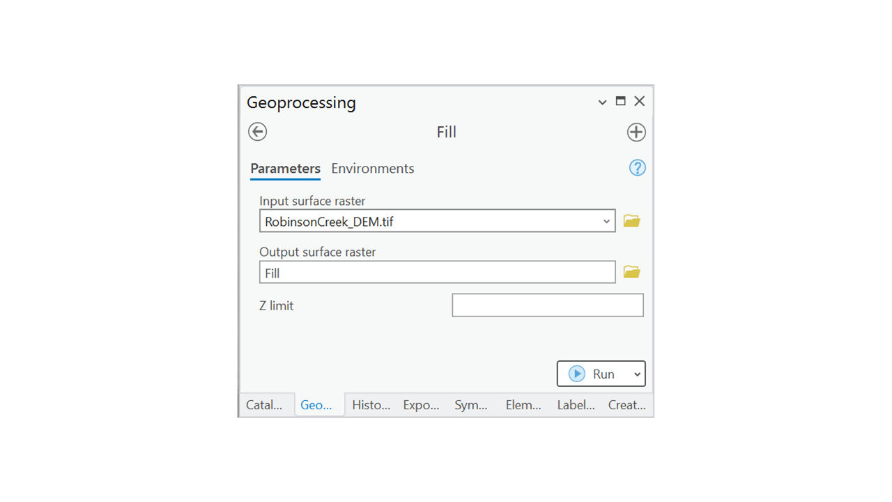

Fig. 93 Fill tool parameters#
Click the Environments tab on the tool and find the Parallel Processing Factor. Type 100% as the parallel processing factor.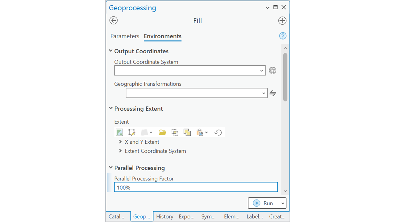

Fig. 94 Fill tool parallel processing factor#

Note: The hydrologic tools are very time consuming in nature. For example, the Fill algorithm requires the program to iteratively fit a 2D plane on top of the DEM to find the sinks and properly fill the sinks up. Whenever there are these iterations in the algorithm for a raster data, it becomes highly computationally expensive. Parallel Processing enables us to utilize the multiple threads in our CPU so that it can be slightly faster. Think of it as the use of multiple cores in GPU for graphics in gaming. However, not all the tools have this options. Putting 100% will use all th threads in yout CPU to run this. From hereon, always try to use 100% as the parallel processing factor in all other hyfrologic tools if possible. This will make your operations faster.
Let’s examine which pixels were filled up. To do that, we can use the Minus (Spatial Analyst) tool to subtract the original DEM from the filled DEM. Name it Fill_Diff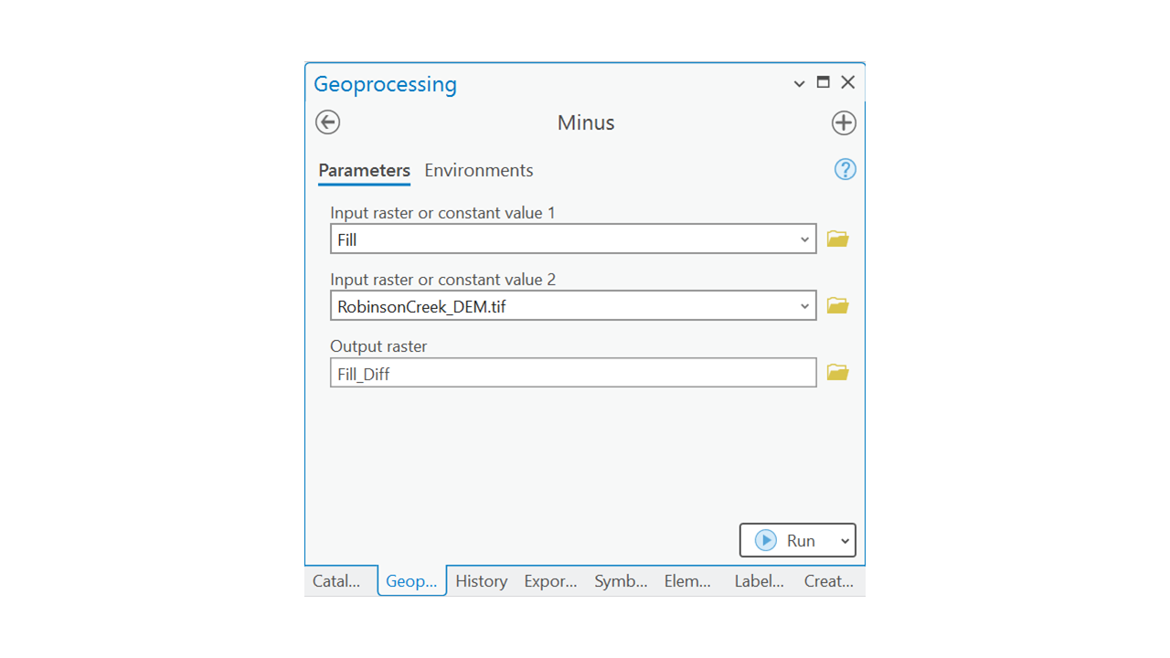

Fig. 95 Fill difference#

Question 1

a. Based on the Fill_Diff raster, you can toggle on and off the Fill raster to see what type of area was filled out. By doing that and examining that, do you see any pattern of the filled portions? To be specific, why do you think the depressions are created? Is it natural or artificial? (Hint: please do not hesitate to ask questions if you are unsure) <2 pt>

Flow direction#

Find Flow Direction (Spatial Analyst) tool and insert the followings as argument. The input would be the Fill DEM, and name the output as FlowDir_D8. Remember to apply parallel processing factor in the Environments.

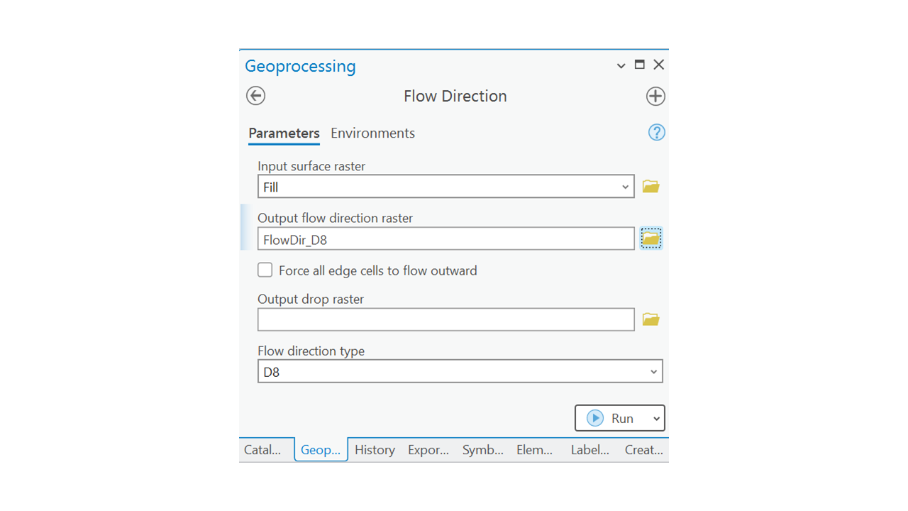
../../_images/fig-4-5.png — Fig. 96 Flow direction#

Flow accumulation#

Find Flow Accumulation (Spatial Analyst) and use the FlowDir_D8 as the input. Name the output FlowAcc_D8 in the geodatabase and remember to use the parallel processing. Flow accumulation might take a while as its a computationally expensive algorithm.

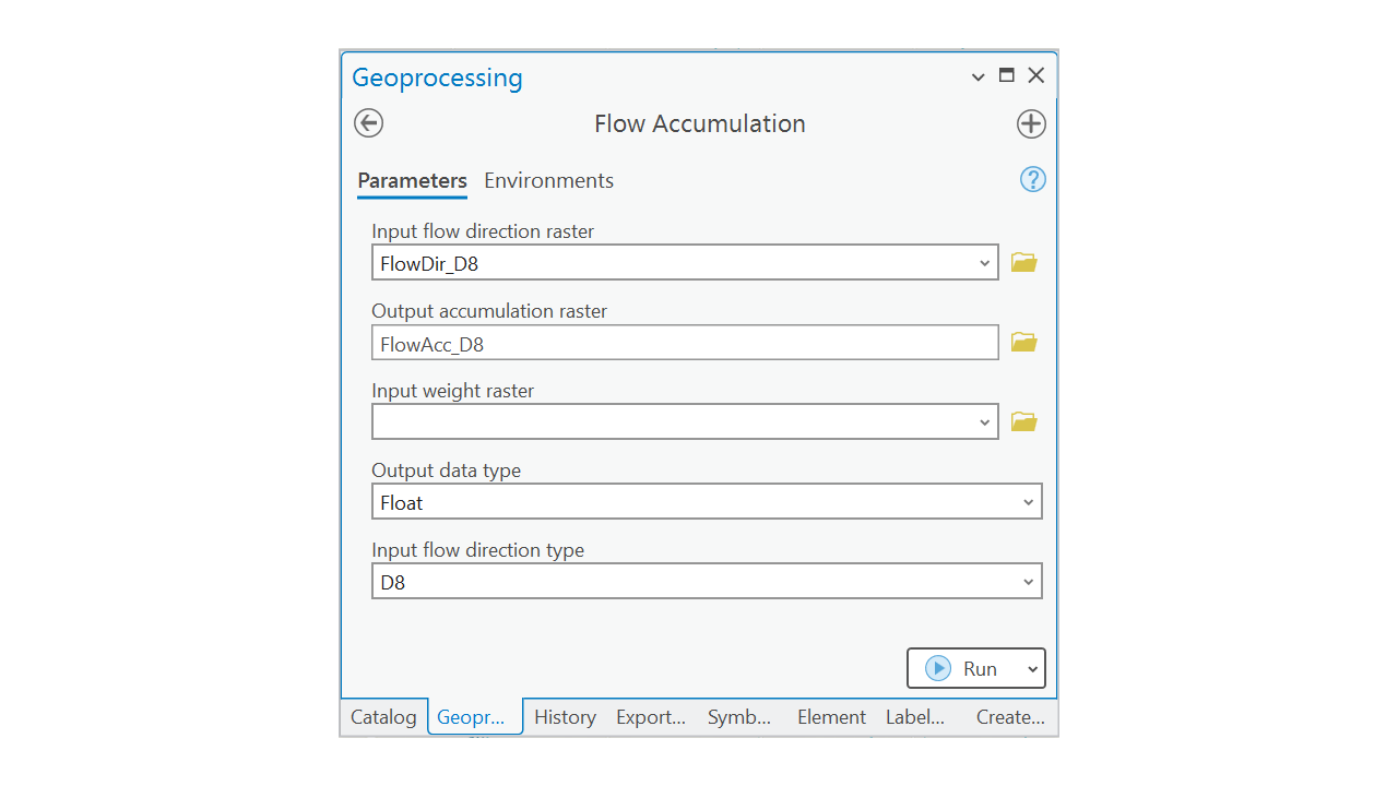
../../_images/fig-4-6.png — Fig. 97 Flow accumulation#

Stream raster#

The flow accumulation raster shows us the number of cells that pours water into each cell. A value of 0 for a cell would mean that no other cell has contributed any water. We can assume that any cell with more that 100 can be a potential cell for a stream. So we can apply a condition to the FlowAcc_D8 raster that if any cell’s value is >= 100, then it is a stream cell and if it’s not then its a NoData.

Find Con (Spatial Analyst) and use the parameters properly. “Con” stands for condition. Name the output as StreamRaster. The true value would be 1, which means if the condition is satisfied for a cell, then the value would be 1, otherwise it would be NoData. Since you have not provided any value to the false constant value, it would indicate we want NoData for these cells.

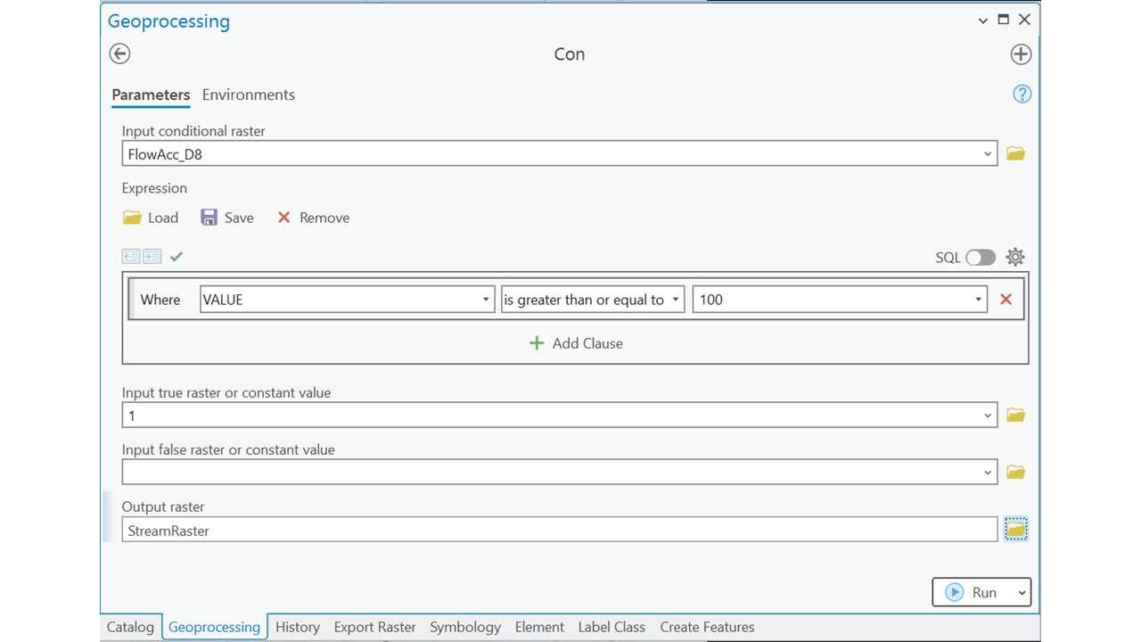
../../_images/fig-4-7.png — Fig. 98 Stream raster using Con#

Question 2

a. Now that you know how to use the Con tool, find out how much area in Square Meters were filled in the Fill process? (Hint: Well! Since I have asked the question here instead before, you know which tool to use. Also remember that the resolution is 10 meters for this DEM.) <3 pt>
b. Explain how you calculated it. <3 pt>

Stream order#

Stream order is a way of classifying the hierarchy of streams in a river system. It starts with the smallest streams, called first-order streams, which have no tributaries. When two first-order streams meet, they form a second-order stream. When two second-order streams meet, they form a third-order stream, and so on. Higher-order streams represent larger and more complex river systems.

Find Stream Order (Spatial Analyst) and use the StreamRaster as Input stream raster and FlowDir_D8 as the Input flow direction raster. Name the output raster as StreamOrder

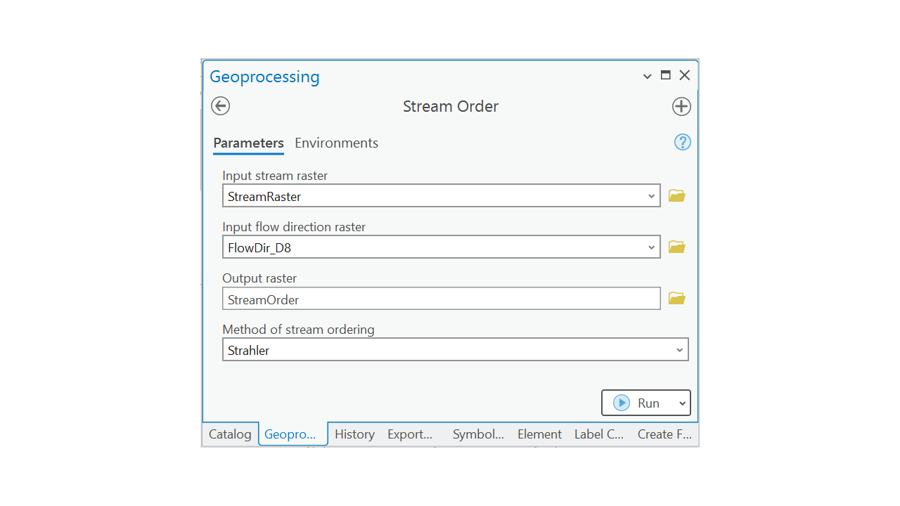
../../_images/fig-4-8.png — Fig. 99 Stream order#

The output raster should have different color coded values which represents the Strahler stream orders.

Stream polyline#

We often need stream lines or drainage systems as polylines instead of rasters. Find Stream to Feature (Spatial Analyst). Use the following parameters as input and output. You could also use the StreamRaster as input for this tool. But that would not give us the stream order information.

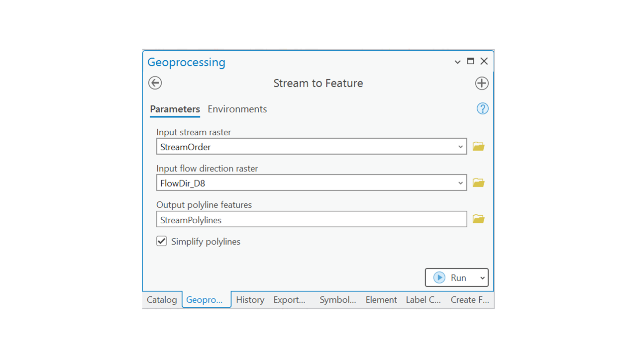
../../_images/fig-4-9.png — Fig. 100 Stream to feature#

Examine the attribute table of the StreamPolylines. Notice that the column grid_code is the column that holds the stream order degree information. 1 means 1st order streams, 2 means 2nd order and so on.

Watershed delineation#

Import the PourPoint faeture into the map.
We want find the area that contributes all the water downnstream through the PourPoint
Find the Watershed (Spatial Analyst) tool. Use the following parameters as input and output. Remember to use the parallel processing factor.

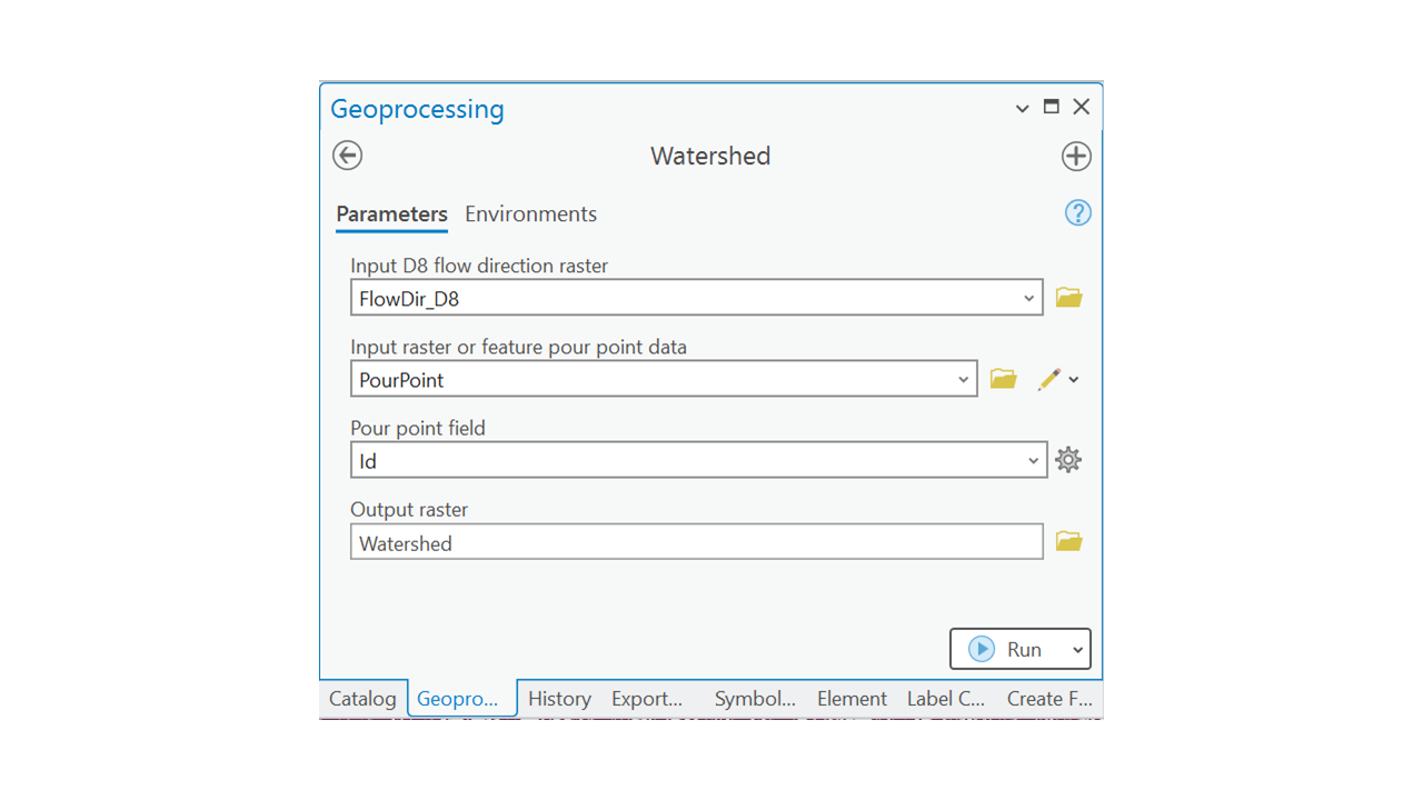
Fig. 101 Watershed#
This would result in a raster data with 0 values and NoData where the areas with 0 values means the watershed for the PourPoint. This is vecause we used the Id as the Pour point field in the Watershed tool and all the values are 0 as the Id was 0 for the point. If we had multiple points, there would be multiple values clustered together within the output raster. Now we can convert the raster to a polygon.
Find Raster to Polygon (Conversion) tool and convert the Watershed raster to a polygon feature named Watershed_Polygon.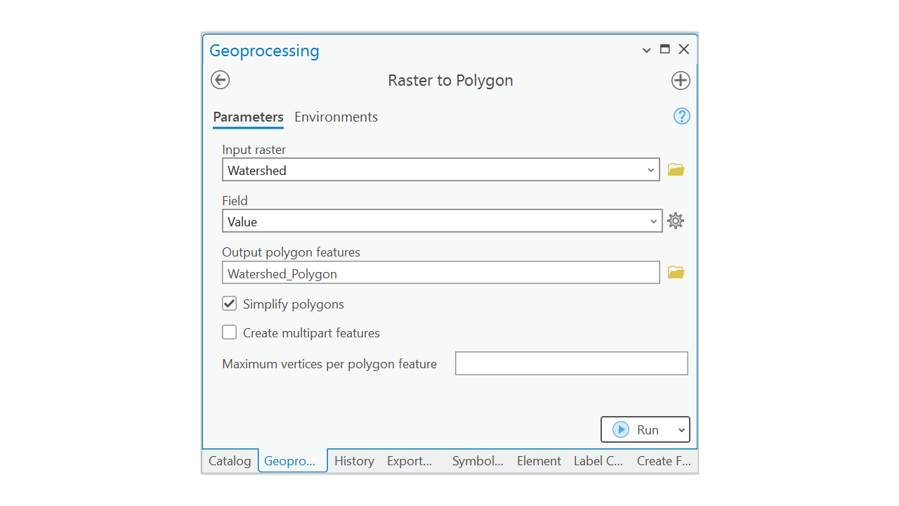

Develop the deliverables#

Question 3

a. Clip the StreamPolylines using the Watershed_Polygon to get only the streams within the delineated watershed. (Hint: Use Clip (Analysis). If you are confused about what would be the input feature and clip feature, please read the documentaion in the link or raise question.) <3 pt>
b. Create a feature class for the streams with the 5th or higher stream order. (Hint: grid_code is the column that has the stream order information) <3 pt>
c. Calculate the length of streams (in Kilo Meters) for each stream order class. Create a table with the columns Stream Order and Length (Kilo Meters), there should be 5 rows for this table. (Hint: Dissolve) <5 pt>
d. What is the area of the watershed boundary in Sq. Km? (Hint: there could be multiple polygons created, just consider the largest polygon’s area) <1 pt>
d. Create a map of the Robinson Creek Watershed with the watershed boundary, streams with order >= 5 (different colors for different streams, use thicker lines for higher order streams and thinner lines for lower order streams), the outlet location. Use other necessary map features. <5 pt>

Answers#

Question 1

a. Because of the roads. These are mostly artificial depressions.